Bias Correction Example
[2]:
import matplotlib.pyplot as plt
import numpy as np
import poligrain as plg
import xarray as xr

from pypwsqc import bias_correction as bc
---------------------------------------------------------------------------
ImportError                               Traceback (most recent call last)
Cell In[2], line 6
      3 import poligrain as plg
      4 import xarray as xr
----> 6 from pypwsqc import bias_correction as bc

ImportError: cannot import name 'bias_correction' from 'pypwsqc' (/home/IWS/seidel/miniconda3/envs/opensense_training/lib/python3.11/site-packages/pypwsqc/__init__.py)
Data download and preparation
In this example, we use an open PWS dataset from Amsterdam published by de Vos et al. (2019). By running the cell below, a NetCDF-file will be downloaded to your current repository (if your machine is connected to the internet).
[9]:
!curl -OL https://github.com/OpenSenseAction/OS_data_format_conventions/raw/main/notebooks/data/OpenSense_PWS_example_format_data.nc
  % Total    % Received % Xferd  Average Speed   Time    Time     Time  Current
                                 Dload  Upload   Total   Spent    Left  Speed
  0     0    0     0    0     0      0      0 --:--:-- --:--:-- --:--:--     0
100 5687k  100 5687k    0     0  19.4M      0 --:--:-- --:--:-- --:--:-- 19.4M
Load the PWS data set
[10]:
ds_pws_orig = xr.open_dataset("OpenSense_PWS_example_format_data.nc")
ds_pws_orig.load()
[10]:
<xarray.Dataset> Size: 237MB
Dimensions:    (time: 219168, id: 134)
Coordinates:
  * time       (time) datetime64[ns] 2MB 2016-05-01T00:05:00 ... 2018-06-01
  * id         (id) <U6 3kB 'ams1' 'ams2' 'ams3' ... 'ams132' 'ams133' 'ams134'
    elevation  (id) <U3 2kB 'nan' 'nan' 'nan' 'nan' ... 'nan' 'nan' 'nan' 'nan'
    latitude   (id) float64 1kB 52.31 52.3 52.31 52.35 ... 52.43 52.3 52.26
    longitude  (id) float64 1kB 4.671 4.675 4.677 4.678 ... 5.036 5.041 5.045
Data variables:
    rainfall   (id, time) float64 235MB 0.0 0.0 0.0 0.0 0.0 ... nan 0.0 0.0 0.0
Attributes:
    title:                 PWS data from Amsterdam
    file author:           Maximilian Graf
    institution:           Wageningen University and Research, Department of ...
    date:                  2022-10-18 10:32:00
    source:                Netamo PWS
    history:               Data derived and reformated from the originally pu...
    naming convention:     OpenSense-0.1
    license restrictions:  CC-BY 4.0 https://creativecommons.org/licenses/by/...
    reference:             https://doi.org/10.1029/2019GL083731
comment: This package handles rainfall data as xarray Datasets. The data set must have time and id dimensions, latitude and longitude as coordinates, and rainfall as data variable.
An example of how to convert .csv data to a xarray dataset is found here.
Aggregate PWS data to hourly values
For this bias correction example, we will aggregate the PWS data to hourly values
For the aggreation, the new value for an hour is considered as valid if at least 10 out 12 5-min values within one hour have valid data. This can be set by the min count parameter.
[ ]:
%%time
ds_pws = ds_pws_orig.resample(time="1h").sum(min_count=10)
CPU times: user 9.77 s, sys: 124 ms, total: 9.9 s
Wall time: 10.2 s
Add cartesian coordinates to dataset using poligrain tools
[12]:
# if lat /lon instead of latitude/longitude
ds_pws.coords["x"], ds_pws.coords["y"] = plg.spatial.project_point_coordinates(
    ds_pws.longitude,
    ds_pws.latitude,
    target_projection="EPSG:25831",
)
Let’s look at the first PWS station in the data set, now with x and y coordinates
[13]:
ds_pws.isel(id=0)
[13]:
<xarray.Dataset> Size: 292kB
Dimensions:    (time: 18265)
Coordinates:
    id         <U6 24B 'ams1'
    elevation  <U3 12B 'nan'
    latitude   float64 8B 52.31
    longitude  float64 8B 4.671
  * time       (time) datetime64[ns] 146kB 2016-05-01 ... 2018-06-01
    x          float64 8B 6.139e+05
    y          float64 8B 5.796e+06
Data variables:
    rainfall   (time) float64 146kB 0.0 0.0 0.0 0.0 0.0 ... 0.0 0.0 0.0 0.0 nan
Attributes:
    title:                 PWS data from Amsterdam
    file author:           Maximilian Graf
    institution:           Wageningen University and Research, Department of ...
    date:                  2022-10-18 10:32:00
    source:                Netamo PWS
    history:               Data derived and reformated from the originally pu...
    naming convention:     OpenSense-0.1
    license restrictions:  CC-BY 4.0 https://creativecommons.org/licenses/by/...
    reference:             https://doi.org/10.1029/2019GL083731
comment: Load reference data set
The bias correction is done by using a quantile mapping based on gamma funtions. For this we need a referecence data. In this example 20 randomly chosen time series from pixels from the gauge-adjusteed KNMI radar product over the Amsterdam Metropolitan area are used as reference for the bias correction. The following cell loads this data set and adds cartesian coordinates as shown above.
[14]:
# path needs to be changed for github
ds_ref = xr.open_dataset("./data/RadarRef_AMS.nc")
ds_ref.load()
ds_ref.coords["x"], ds_ref.coords["y"] = plg.spatial.project_point_coordinates(
    ds_ref.lon,
    ds_ref.lat,
    target_projection="EPSG:25831",
)
Selecting the nearest reference station
In this example, we want to bias correct the data from the PWS ‘ams65’ First we look for the closest neighbor in the reference data set
[15]:
pws_id = "ams65"
# use poligrain tool to find nearest neighbor.
max_distance = 25e3
closest_neighbor = plg.spatial.get_closest_points_to_point(
    ds_points=ds_pws.sel(id=pws_id),
    ds_points_neighbors=ds_ref,
    max_distance=max_distance,
    n_closest=1,
)
closest_neighbor
[15]:
<xarray.Dataset> Size: 40B
Dimensions:      (id: 1, n_closest: 1)
Coordinates:
  * id           (id) <U6 24B 'ams65'
Dimensions without coordinates: n_closest
Data variables:
    distance     (id, n_closest) float64 8B 784.0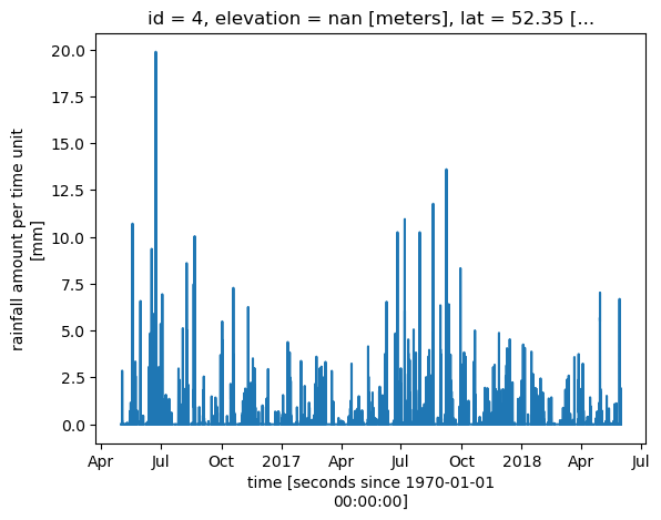
neighbor_id (id, n_closest) object 8B '4'Plot time series for reference data
[16]:
ref_id = str(closest_neighbor.neighbor_id.data[0][0])
ds_ref.sel(id=ref_id).rainfall.plot()
[16]:
[<matplotlib.lines.Line2D at 0x7f098eab6950>]
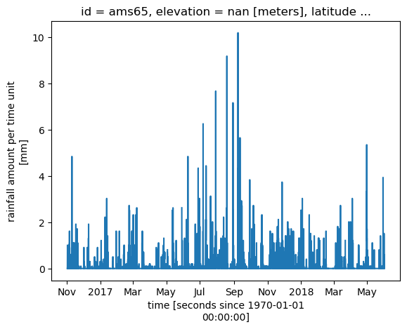
Plot time series for selected PWS
[17]:
ds_pws.sel(id=pws_id).rainfall.plot()
[17]:
[<matplotlib.lines.Line2D at 0x7f0980041c50>]
Convert data to np.array
[18]:
ref = ds_ref.sel(id=ref_id).rainfall.data
pws = ds_pws.sel(id=pws_id).rainfall.data
Fitting data to a theoretical gamma distribution
Fit theoretical gamma distribution to the PWS and the reference data. Since rainfall data is highly skewed, we only fit the data above a certain threshold (here 1mm) and treat the values between 0mm and the threshold as censored values
[ ]:
shape_ref, scale_ref, p0_ref = bc.fit_gamma_params_with_threshold(ref, 1)
print(
    f"Optimal parameters: shape = {shape_ref:.5f}, scale = {scale_ref:.5f}, p0 = {p0_ref:.2f}"
)
Fit parameters for reference
[ ]:
shape_ref, scale_ref, p0_ref = bc.fit_gamma_params_with_threshold(ref, 1)
print(
    f"Optimal parameters: shape = {shape_ref:.5f}, scale = {scale_ref:.5f}, p0 = {p0_ref:.2f}"
)
Optimal parameters: shape = 0.26362, scale = 2.12160, p0 = 0.83
Fit parameters for PWS
[ ]:
shape_pws, scale_pws, p0_pws = bc.fit_gamma_params_with_threshold(pws, 1)
print(
    f"Optimal parameters: shape = {shape_pws:.5f}, scale = {scale_pws:.5f}, p0 = {p0_pws:.2f}"
)
Optimal parameters: shape = 0.49763, scale = 0.98254, p0 = 0.85
Do the bias correction using quantile mapping
[21]:
pws_corr = bc.qq_gamma(pws, shape_pws, scale_pws, p0_pws, shape_ref, scale_ref, p0_ref)
Create a new xr.Dataset for the selected PWS
[22]:
selected_pws = ds_pws.sel(id=pws_id)
[23]:
selected_pws
[23]:
<xarray.Dataset> Size: 292kB
Dimensions:    (time: 18265)
Coordinates:
    id         <U6 24B 'ams65'
    elevation  <U3 12B 'nan'
    latitude   float64 8B 52.35
    longitude  float64 8B 4.885
  * time       (time) datetime64[ns] 146kB 2016-05-01 ... 2018-06-01
    x          float64 8B 6.284e+05
    y          float64 8B 5.801e+06
Data variables:
    rainfall   (time) float64 146kB nan nan nan nan nan ... 0.0 0.0 0.0 0.0 nan
Attributes:
    title:                 PWS data from Amsterdam
    file author:           Maximilian Graf
    institution:           Wageningen University and Research, Department of ...
    date:                  2022-10-18 10:32:00
    source:                Netamo PWS
    history:               Data derived and reformated from the originally pu...
    naming convention:     OpenSense-0.1
    license restrictions:  CC-BY 4.0 https://creativecommons.org/licenses/by/...
    reference:             https://doi.org/10.1029/2019GL083731
comment: Add the bias corrected values as new data variable to the existing xr.Dataset
[24]:
var_dim = ds_pws.rainfall.shape
rainfall_bcorr = np.full(var_dim, np.nan)
# dimensions might be swapped which causes an error. Transpose (rainfall_bcorr.T) is a first fix for this
selected_pws["rainfall_biascorr"] = (selected_pws["rainfall"].dims, pws_corr)
Check for first valid entry in PWS rainfall data and define start and end dates for comparison plots
[25]:
first_valid_index = selected_pws.rainfall.notnull().argmax(dim="time")
start_date = selected_pws.time.isel(time=first_valid_index)
end_date = str(selected_pws.time.data[-1])
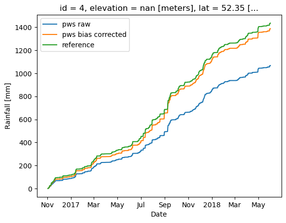
Plot original and bias corrected cumulatice rainfall sums for the selected PWS
[26]:
selected_pws.rainfall.sel(time=slice(start_date, end_date)).cumsum().plot(
    label="pws raw"
)
selected_pws.rainfall_biascorr.sel(time=slice(start_date, end_date)).cumsum().plot(
    label="pws bias corrected"
)
ds_ref.sel(id=ref_id).rainfall.sel(time=slice(start_date, end_date)).cumsum().plot(
    label="reference"
)
plt.legend()
plt.ylabel("Rainfall [mm]")
plt.xlabel("Date")
;
[26]:
''
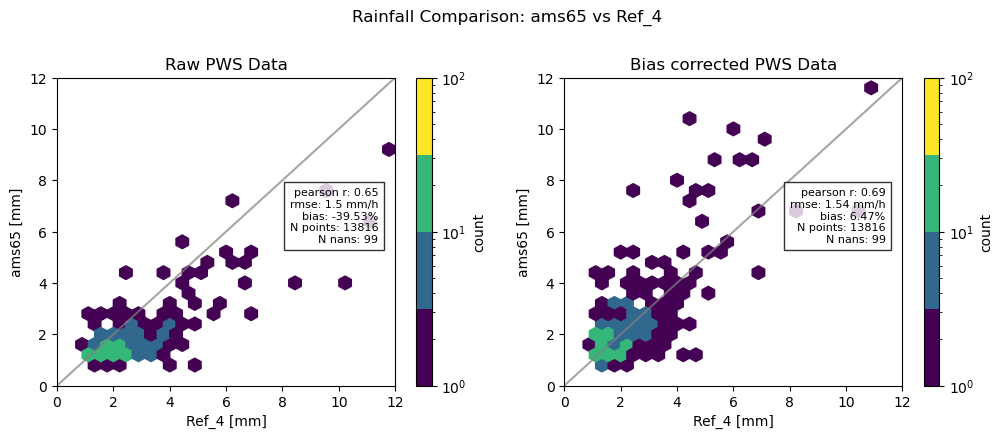
Plot Hexbinplot coparison with reference before and after bias correction
[ ]:
threshold = 1
da_pws_raw = selected_pws.rainfall.sel(time=slice(start_date, end_date)).data.flatten()[
    :-1
]
da_pws_biascorr = selected_pws.rainfall_biascorr.sel(
    time=slice(start_date, end_date)
).data.flatten()[:-1]
da_ref = (
    ds_ref.sel(id=ref_id).rainfall.sel(time=slice(start_date, end_date)).data.flatten()
)

rainfall_metrics = plg.validation.calculate_rainfall_metrics(
    reference=da_ref,
    estimate=da_pws_raw,
    ref_thresh=threshold,
    est_thresh=threshold,
)
rainfall_metrics_1 = plg.validation.calculate_rainfall_metrics(
    reference=da_ref,
    estimate=da_pws_biascorr,
    ref_thresh=threshold,
    est_thresh=threshold,
)
# plotting the scatter density plots
fig, ax = plt.subplots(1, 2, figsize=(12, 4))
fig.suptitle(f"Rainfall Comparison: {pws_id} vs Ref_{ref_id}", fontsize=12, y=1.05)
hx = plg.validation.plot_hexbin(
    da_ref,
    da_pws_raw,
    ref_thresh=threshold,
    est_thresh=threshold,
    # extent=[0,11,0,11],
    ax=ax[0],
)
ax[0].set_title("Raw PWS Data")
ax[0].set_xlabel("Ref_" + ref_id + " [mm]")
ax[0].set_ylabel(pws_id + " [mm]")
hx = plg.validation.plot_hexbin(
    da_ref,
    da_pws_biascorr,
    ref_thresh=threshold,
    est_thresh=threshold,
    # extent=[0,11,0,11],
    ax=ax[1],
)
ax[1].set_title("Bias corrected PWS Data")
ax[1].set_xlabel("Ref_" + ref_id + " [mm]")
ax[1].set_ylabel(pws_id + " [mm]")
# adding metrics to the plot for subplot 0
plotted_metrics = (
    f"pearson r: {np.round(rainfall_metrics['pearson_correlation_coefficient'], 2)}\n"
    f"rmse: {np.round(rainfall_metrics['root_mean_square_error'], 2)} mm/h\n"
    f"bias: {np.round(rainfall_metrics['percent_bias'], 2)}%\n"
    f"N points: {rainfall_metrics['N_all']}\n"
    f"N nans: {rainfall_metrics['N_nan']}"
)
ax[0].text(
    0.95,
    0.55,
    plotted_metrics,
    fontsize=8,
    transform=ax[0].transAxes,
    verticalalignment="center",
    horizontalalignment="right",
    bbox={"facecolor": "white", "alpha": 0.8},
)
# adding metrics to the plot for subplot 1
plotted_metrics_1 = (
    f"pearson r: {np.round(rainfall_metrics_1['pearson_correlation_coefficient'], 2)}\n"
    f"rmse: {np.round(rainfall_metrics_1['root_mean_square_error'], 2)} mm/h\n"
    f"bias: {np.round(rainfall_metrics_1['percent_bias'], 2)}%\n"
    f"N points: {rainfall_metrics_1['N_all']}\n"
    f"N nans: {rainfall_metrics_1['N_nan']}"
)
ax[1].text(
    0.95,
    0.55,
    plotted_metrics_1,
    fontsize=8,
    transform=ax[1].transAxes,
    verticalalignment="center",
    horizontalalignment="right",
    bbox={"facecolor": "white", "alpha": 0.8},
)
ax[0].set_xlim(0, 12)
ax[0].set_ylim(0, 12)
ax[1].set_xlim(0, 12)
ax[1].set_ylim(0, 12)
;
''